A discrete event simulator in PHP

How do you test code designed to run on a large and expensive computing cluster? How do you reproduce complex, time-dependent emergent behaviour of a cluster of network components?

A discrete event simulation is like the event loop you find in asynchronous applications, but simplified. Instead of waiting on all sorts of file descriptors, there is only a simulated “sleep” operation, which wakes up at a specified time.

I built an event simulator in PHP and used it to test 5000 lines of unmodified production code.

I used PHP’s fibers to avoid the need to rewrite the code into an asynchronous event-driven pattern. Fibers are like threads in that they have their own stack, but they are run in a single physical process and are only suspended when they request it. Fibers allow a kind of cooperative multitasking.

When the code under test wants to do a database query, a mock database subclass does a simulated sleep and then returns.

public function query( $sql ) {
    $this->eventLoop->sleep( 0.1 );
    return new FakeResultWrapper( [] );
}

The simulated sleep queues an event in the future, then suspends the currently running fiber. The event loop then gets the next event (the one with the lowest timestamp), sets the current timestamp to the one specified in the event, and resumes the event’s fiber.

If the code under test wants to know the current time, we have to arrange for it to get the simulated time from the event loop. But the relevant classes already had a way to do this, to support unit testing.

To start up a new simulated thread, like a request being handled, we make a new fiber and run a function in the context of that fiber. The time between requests follows an exponential distribution, just like uncorrelated events in reality.

public function makeRequests() {
    while ( true ) {
        $delay = RandomDistribution::exponential( $this->rate );
        $this->eventLoop->sleep( $delay );
        $this->eventLoop->addTask( [ $this, 'handleRequest' ] );
    }
}
 
public function handleRequest() {
    $client = $this->getRandomClient();
    $db = $client->getLoadBalancer()->getConnection( DB_REPLICA );
    $db->query( 'SELECT do_work()' );
}

This was easy and worked surprisingly well. The main challenge was dealing with the large amount of data generated by the simulation. I added a set of metrics classes and a system for writing their state to a CSV file. I used a spreadsheet to process and plot the data.

Administrative tasks, like reporting the current state of the metrics, are also done using fibers.

public function report() {
    while ( true ) {
        $this->recordTimeStep();
        $this->eventLoop->sleep( $this->timeStep );
    }
}

To terminate the simulation, we throw an exception in every fiber.

private function terminateFibers() {
    foreach ( $this->fibers as $fiber ) {
        if ( $fiber->isSuspended() ) {
            try {
                $fiber->throw( new TerminateException );
            } catch ( TerminateException $e ) {}
        }
    }
}

The scenario I tested has 139 application hosts serving about 7500 requests per second. The application tries to balance load across 11 replica database hosts, which have latency and configured load weights derived from production data. I can inject fault conditions and see how the load is rebalanced.

This scenario typically has about 800 fibers active at any given time. This only requires a few hundred megabytes of RAM, so I can comfortably run it on my laptop. It takes about 6 seconds of real time to run 1 second of simulated time.

A chart with lines showing active connection count versus time for four database servers.
A sample of the simulator’s output data.

Hey that’s cool. I want to use your event simulator for my thing.

If you’re working on MediaWiki, contact me and we’ll talk about your needs.

If you’re working on some other thing and need a generic event simulator for PHP, please study my code and either fork it or use it for inspiration. Ideally turn it into a nice Composer library and let me know when it is ready for everyone to use.

Xdebug on demand

My MediaWiki test instance normally runs without Xdebug, since that gives good performance. But when I request a debug session in PHPStorm, Xdebug is automatically enabled.

I don’t often share config snippets since they are so specific to the way I have things set up. You will most likely have to adapt this to your situation. But at least it should help you to know that conditionally enabling Xdebug is possible.

I use PHP-FPM which, unlike Apache mod-php, allows you to run multiple versions of PHP. I use Apache to detect Xdebug’s cookie or query string. Then I have a separate instance of PHP-FPM just for Xdebug, with a separate php.ini.

I’m using Xdebug 3.0. I upgraded from Xdebug 2 for this project since I figured there is no point putting a lot of effort into an Xdebug 2 installation which I would almost certainly have to upgrade within a year.

I have a file called /etc/apache2/php.conf along the lines of:

<FilesMatch ".+\.php$">
	<If "%{HTTP_COOKIE} =~ /XDEBUG_SESSION/ || %{QUERY_STRING} =~ /XDEBUG_SESSION_START=/ || %{REQUEST_URI} =~ /intellij_phpdebug_validator/">
		SetHandler "proxy:unix:/run/php/php8.0-fpm-xdebug.sock|fcgi://localhost"
	</If>
	<Else>
		SetHandler "proxy:unix:/run/php/php8.0-fpm.sock|fcgi://localhost"
	</Else>
</FilesMatch>

I include that into any VirtualHost directives that need PHP execution.

<VirtualHost *:443>
	ServerName test.internal
	...
	Include php.conf
</VirtualHost>

The non-Xdebug instance of PHP-FPM is installed in the usual way, in my case using OndÅ™ej Surý’s PPA. I copied the systemd service file for PHP-FPM from /lib/systemd/system/php8.0-fpm.service to /etc/systemd/system/php-fpm-xdebug.service and changed the paths to avoid conflicts:

[Unit]
Description=The PHP 8.0 FastCGI Process Manager (with xdebug)
Documentation=man:php-fpm8.0(8)
After=network.target

[Service]
Type=notify
ExecStart=/usr/sbin/php-fpm8.0 --nodaemonize --fpm-config /etc/php/8.0/fpm-xdebug/php-fpm.conf -c /etc/php/8.0/fpm-xdebug
ExecStartPost=-/usr/lib/php/php-fpm-socket-helper install /run/php/php-fpm-xdebug.sock /etc/php/8.0/fpm-xdebug/pool.d/www.conf 80
ExecStopPost=-/usr/lib/php/php-fpm-socket-helper remove /run/php/php-fpm-xdebug.sock /etc/php/8.0/fpm-xdebug/pool.d/www.conf 80
ExecReload=/bin/kill -USR2 $MAINPID

[Install]
WantedBy=multi-user.target

/etc/php/8.0/fpm-xdebug is the configuration directory for the new instance of PHP-FPM, initially based on a copy of /etc/php/8.0/fpm. To avoid loading Xdebug into the non-Xdebug instance, I commented out the zend_extension line in /etc/php/8.0/mods-available/xdebug.ini , since the package has a bug which recreates the conf.d symlinks if you delete them.

I don’t usually use the default php.ini, I just wipe it after package installation and start with an empty file, since that makes it easier to see which defaults I’ve overridden. You lose the documentation comments, but I’m able to read the manual, so that’s fine.

My /etc/php/8.0/fpm-xdebug/php.ini has:

zend_extension = xdebug.so
xdebug.mode = debug
xdebug.client_host = 169.254.1.1

Replace 169.254.1.1 with the address of the host on which your IDE runs, as seen by the container. I am using systemd-nspawn with bridged networking, which allows PHP to connect to the host using link-local addresses.

A few more little things to avoid conflicts with the main PHP-FPM instance. Like php.ini, I started with empty files, not default files. /etc/php/8.0/fpm-xdebug/php-fpm.conf contains only:

[global]
pid = /run/php/php8.0-fpm-xdebug.pid
error_log = /var/log/php8.0-fpm-xdebug.log

include=/etc/php/8.0/fpm-xdebug/pool.d/*.conf

And /etc/php/8.0/fpm-xdebug/pool.d/www.conf:

[www]
user = www-data
group = www-data
listen = /run/php/php8.0-fpm-xdebug.sock
listen.owner = www-data
listen.group = www-data
pm = dynamic
pm.max_children = 5
pm.start_servers = 1
pm.min_spare_servers = 1
pm.max_spare_servers = 3

I think that’s it. Now it should just be a matter of

systemctl daemon-reload
systemctl start php-fpm-xdebug
systemctl enable php-fpm-xdebug
systemctl reload apache2

To debug a web request, set a breakpoint, then in Run > Edit Configurations, create a “PHP Web Page” configuration. The URL you use here does not have to be the exact one you want to debug, it just has to be in the same cookie domain. Then Run > Debug… and select the configuration. This will spawn a browser tab which activates Xdebug with the XDEBUG_SESSION_START query string parameter. Xdebug modifies the response to set the XDEBUG_SESSION cookie.

Since XDebug 3.1, the cookie has no expiry time set, but you can append XDEBUG_SESSION_STOP=1 to the query string to cause it to remove its session cookie. With no session cookie, you will automatically be back to PHP without Xdebug.

You can get PHPStorm to run command-line scripts via SSH, but I find it’s most convenient to run them in the usual way, with the PHPStorm option “Listen for PHP Debug Connections” enabled.

I use a shell script wrapper along the lines of:

XDEBUG_TRIGGER=1 PHP_IDE_CONFIG=serverName=test.internal \
  php -dzend_extension=xdebug.so -dxdebug.mode=debug -dxdebug.client_port=9000 \
  -dxdebug.client_host=169.254.1.1 "$@"

The serverName configuration variable here is necessary to select the right path mappings — it must correspond to the name of the server in PHPStorm’s File > Settings > PHP > Servers.

The waste-to-energy offset scam

Growing plants and then burying them or incorporating them into soil is one of the few practical and efficient things we can do to remove CO2 from the atmosphere and permanently store it. Agricultural wastes such as rice husks, when incorporated into soil at the site of production, readily mineralize, becoming encased in silica, preventing decomposition. It’s estimated that in India, crop wastes produce about 87 million tonnes of mineralized carbon per year. 1

I’ve been reading about carbon offsets lately, as a way to reduce Wikimedia Foundation’s impact on the environment. Carbon offsets are produced by an organisation doing some activity which reduces CO2 in the atmosphere. The offsets are independently verified, most notably by the Gold Standard Foundation. Certificates for CO2 abatement are issued and registered in a market.

The Gold Standard Foundation’s website prominently promotes a waste-to-energy project in Chhattisgarh, India as a carbon offset.2 Offsets against this project can be bought directly from Gold Standard for $11 USD/t. The project aimed to divert 145,920t per annum of rice husks, which otherwise would have been disposed of at the place of production, and to burn them for energy instead. In an attempt to figure out how Gold Standard could justify endorsing this project, I read its Project Design Document (PDD). 3

The document is rigorous in appearance. It adds up the emissions in the “baseline” case, that is, a model for what would have happened if the project was not built. Then it adds up emissions in the “project” case. The difference between these is the carbon offset value.

The baseline case has emissions of 110,881 tCO2e per year, due to electricity generated by the existing mix of generators. 4. In the project case, the emissions are only 3,372 tCO2e per year, mostly due to off-site processing of the rice husks and on-site methane emissions. 5. The emissions due to actually burning the rice husks for energy are supposedly zero — such emissions are dismissed with the phrase “It is assumed that CO2 emissions from surplus biomass residues do not lead to changes of carbon pools in the LULUCF [land use, land-use change, and forestry] sector”.6

This is quite a heroic assumption. If this was new agricultural production, using completely unproductive land (like a desert), you could see how the emissions from burning the plants would be absorbed again by the next year’s crop. But for rice waste which was previously discarded, this is patently not the case. The carbon is diverted from permanent storage in the ground to CO2 emissions in the air, a description which could equally apply to fossil fuels.

Could it be that methane emissions from on-site rice husk dumps are assumed to neatly cancel out the emissions from burning the wastes? Or perhaps was most of the rice was previously burnt by the farmer? No, the PDD conservatively assumes that the total emissions in the baseline case due to decomposition and burning is zero.7

If we adopt these conservative assumptions, but estimate the amount of CO2 actually released by burning rice husks for electricity, the sign of the carbon offset is reversed. That is to say, burning rice husks appears to emit more carbon per unit of electricity than the existing mix of generators. Assuming that rice husks are 38% carbon,8 burning 145,920t of rice husks per annum would release 203,000t of CO2. So the project as a whole would actually increase atmospheric CO2 by 96,000t per annum.

And yet this is being sold as an offset, to absolve wealthy individuals and corporations of their responsibility for emitting yet more CO2!

I set out this entire case to the Gold Standard Foundation by email. On November 3, 2018, they confirmed that they had received the email and that it had been forwarded to their technical team. No further response has been received as of November 12.

Update

The Gold Standard Foundation provided the following response. Essentially they claim that methane emissions from on-site rice husk dumps do indeed cancel out emissions from burning those rice husks for power. I don’t believe this has a firm scientific basis and look forward to a more rigorous approach in future.

The non-fossilized and biodegradable organic material originating from plants for example crop residue is considered carbon neutral – due to no net effect on the biosphere’s carbon concentration. Put simply, the combustion of crop residue releases carbon dioxide which in turn is readily absorbed by plants. Through this cycle, the plants remove carbon from the atmosphere, and carbon is released back to the atmosphere when plants are burned. Since, use of the crop residue for energy use is likely substituting the CO2 emissions from fossil fuel, the energy generation from crop residue such as rice husk burning is considered net carbon neutral.

The permanent sequestration of carbon in rice husks depends on what would happen to the dumped rice husks. As you may already know, the dumped husk will decompose – primarily due to the microbial activity – this will cause anaerobic or aerobic decomposition. In the case of an anaerobic situation, similar to a Municipal Solid Waste (MSW) landfill; the decomposition or organic matter leads to methane emissions, a more potent greenhouse gas as compared to CO2 and further, not one that plants can absorb. While in aerobic decomposition, most of the carbon in the organic material (approximately 2/3) is released into the atmosphere as CO2, which is carbon neutral. In both the cases, the eventual decomposition of the rice husk will happen and it will lead to a release of GHGs (CO2 and/or CH4) in the atmosphere rather than permanent sequestration.

The exclusion of emissions from uncontrolled burning and/or decay in aerobic conditions in baseline scenario is assumed 0 and is conservative. The applied GHGs quantification methodology (ACM0018) keeps it optional for the project to consider these emissions. A likely assumption is that the baseline emissions (primarily CH4 emissions only from burning as CO2 is carbon neutral) would be higher due to inefficient burning or decay as compared to the project situation. Therefore, exclusion of emissions from burning in baseline will lead to net lower emission reductions and is conservative.

Also, the GHGs accounting methodology applied in the project requires an assessment of the availability of the risk husks (annually) to capture any diversion (new) of rice husk from other potential uses. It means the emission reductions estimated or verified are based on field studies of rice husk availability. If any change occurs in potential use of the rice husks (in the project situation) this would be captured and accounted for in the emissions reduction calculations.

Finally, the ex-ante emission reductions in the PDD are estimated based on certain assumptions, for example – potential use of surplus biomass, which is further monitored along with the project operation. The project developer via an independent third party annually conducts field studies to estimate the availability of surplus rice husk within a 50km radius of where the project sources its rice husk. These studies, indicate that the project only uses surplus biomass that would have been dumped in the absence of the project and confirms the initial assumption made in the PDD.

  1. Rajendiran, S., Coumar, M. V., Kundu, S., Ajay, Dotaniya, M. L., & Rao, A. S. (2012). Role of phytolith occluded carbon of crop plants for enhancing soil carbon sequestration in agro-ecosystems. Current Science (00113891), 103(8), 911.
  2. https://www.goldstandard.org/projects/20-mw-biomass-power-project-chhattisgarh-india (archive)
  3. https://mer.markit.com/br-reg/services/processDocument/downloadDocumentById/103000000063706
  4. PDD page 38, BEEL,y
  5. PDD page 40, PEy
  6. PDD page 15, “Combustion of biomass residues for electricity generation”
  7. Aerobic decomposition and burning is on PDD page 39, termed BEBR,B1/B3,y. Baseline methane emissions are on page 31, termed BEBR,B2,y.
  8. Thipwimon Chungsangunsit, Shabbir H. Gheewala, Suthum Patumsawad. Emission Assessment of Rice Husk Combustion
    for Power Production. https://waset.org/publications/514/emission-assessment-of-rice-husk-combustion-for-power-production. Adjusting the figure in table 1 to calculate C as a percentage of wet mass.

Laser speckle contrast imaging

When you shine a laser on a wall, the laser light seems to sparkle. A weird, shifting pattern of random dots appears in the illuminated spot. When you move your head, the pattern shifts around, seeming to follow you. The random dots seem to get larger as you move further away from them. This weird effect is called laser speckle. It is caused by interference patterns created when the coherent light strikes a finely textured surface — particularly textures of approximately the same size as the wavelength of light. It is a little window into the microscopic world.

hand-30f-ir8

A loop of 30 infrared image frames captured using a Kinect. Look closely at the hand, you can see the laser speckle pattern change.

If you shine a laser on your hand, the places where more blood is flowing beneath your skin will seem to sparkle more vigorously — changing more often, with a finer-grained pattern. This is because the light is bouncing off your blood cells, and when they move, they cause the speckle pattern to shift around.

You can use a camera to record this, and with computer assistance, quantitatively determine blood flow. This is an established technique in medical diagnosis and research, and is called laser speckle contrast imaging, or LSCI.

An awesome paper by Richards et al written in 2013 1 demonstrated that LSCI could be done with $90 worth of equipment and an ordinary computer, not thousands of dollars as researchers had previously been led to believe. All you need to do is shine a laser pointer, record with a webcam, and compute the local standard deviation either in time or space. I assumed when I first read this about a year ago that hobbyists would be falling over each other to try this out, but this appears to not be the case. I haven’t been able to find any account of amateur LSCI.

The University of Texas team, led by Andrew Dunn, previously provided software for the interpretation of captured images, but this software has been withdrawn and was presumably not open source. Thus, I aim to develop open source tools to capture and analyse laser speckle images. You can see my progress in the GitHub project I have created for this work.

The Wikimedia Foundation have agreed to reimburse reasonable expenses incurred in this project out of their Wellness Program, which also covers employee education and fitness.

Inspiration

My sister Melissa is a proper scientist. I helped her with technical aspects of her PhD project, which involved measuring cognitive bias in dogs using an automated training method.2 I built the electronics and wrote the microcontroller code.

She asked me if I had any ideas for cheap equipment to measure sympathetic nervous system response in dogs. They were already using thermal cameras to measure eye blood flow, but such cameras are very expensive, and she was wondering if a cheaper technique could be used to provide dog owners with insight into the animal’s behaviour. I came across LSCI while researching this topic. I’m not sure if LSCI is feasible for her application, but it has been used to measure the sympathetic vasomotor reflex in humans. 3

Hardware

Initially, I planned to use visible light, with one or two lenses to expand the beam to a safe diameter. Visible light is not ideal for imaging the human body through the skin, since the absorption coefficient of skin falls rapidly in the red and near-infrared region. But it has significant advantages for safety and convenience. The retina has no pain receptors — the blink reflex is triggered by visible light alone. But like visible light, light from a near infrared laser is focused by the eye into a tiny spot on the retina. A 60mW IR laser will burn a hole in your retina in a fraction of a second, and the only sign will be if the retina starts bleeding into the vitreous humour.

I ordered a 100mW red laser on eBay, and then started shopping for cameras, thinking (based on Richards et al) that cameras capable of capturing video in the raw Bayer mode would be easy to come by. In fact, the Logitech utility used by Richards et al is no longer available, and recent Logitech cameras do not appear to support raw image capture.

I’ll briefly explain why raw Bayer mode capture is useful. Camera manufacturers are lying to you about your camera’s resolution. When you buy a 1680×1050 monitor, you expect it to have some 1.7 million pixels each of red, green and blue — 5.3 million in total. But a 1680×1050 camera only has 1.7 million pixels in total, a quarter of them red, a quarter blue, and half green. Then, the camera chipset interpolates this Bayer image data to produce RGB data at the “full” resolution. This is called demosaicing.

Cameras use all sorts of different algorithms for demosaicing, and while we don’t know exactly what algorithm is used in what camera, they all make assumptions about the source image which do not hold for laser speckle data. Throw away the signal, we’re only interested in the noise. Our image is not smoothly-varying, we want to know about sharp variations on the finest possible scale.

Ideally, you would like to use a monochrome camera, but at retail, such cameras are perversely much more expensive than colour cameras. I asked the manufacturer about the technical details of this cheap “B/W” camera. They said it is actually a colour image sensor with the saturation turned down to zero in post-processing firmware!

Enter the Microsoft Kinect. This excellent device is sold with the Microsoft Xbox. I bought one intended for the Xbox 360 (an obsolete model) second hand for $25 AUD plus postage, then replaced the proprietary plug with a standard USB plug and DC power jack.

This device has an IR laser dot pattern projector, an IR camera with a filter matched to the laser, and an RGB camera.  Following successful reverse engineering of the USB protocol in 2010-11, it is now possible to extract IR and raw Bayer image streams from the Kinect’s cameras.

The nice thing about the Kinect’s IR laser is that despite providing about 60mW of optical power output, it has integrated beam expansion, which means the product as a whole is eye-safe. To homogenize the dot pattern, you don’t need lenses, you can just use a static diffuser.

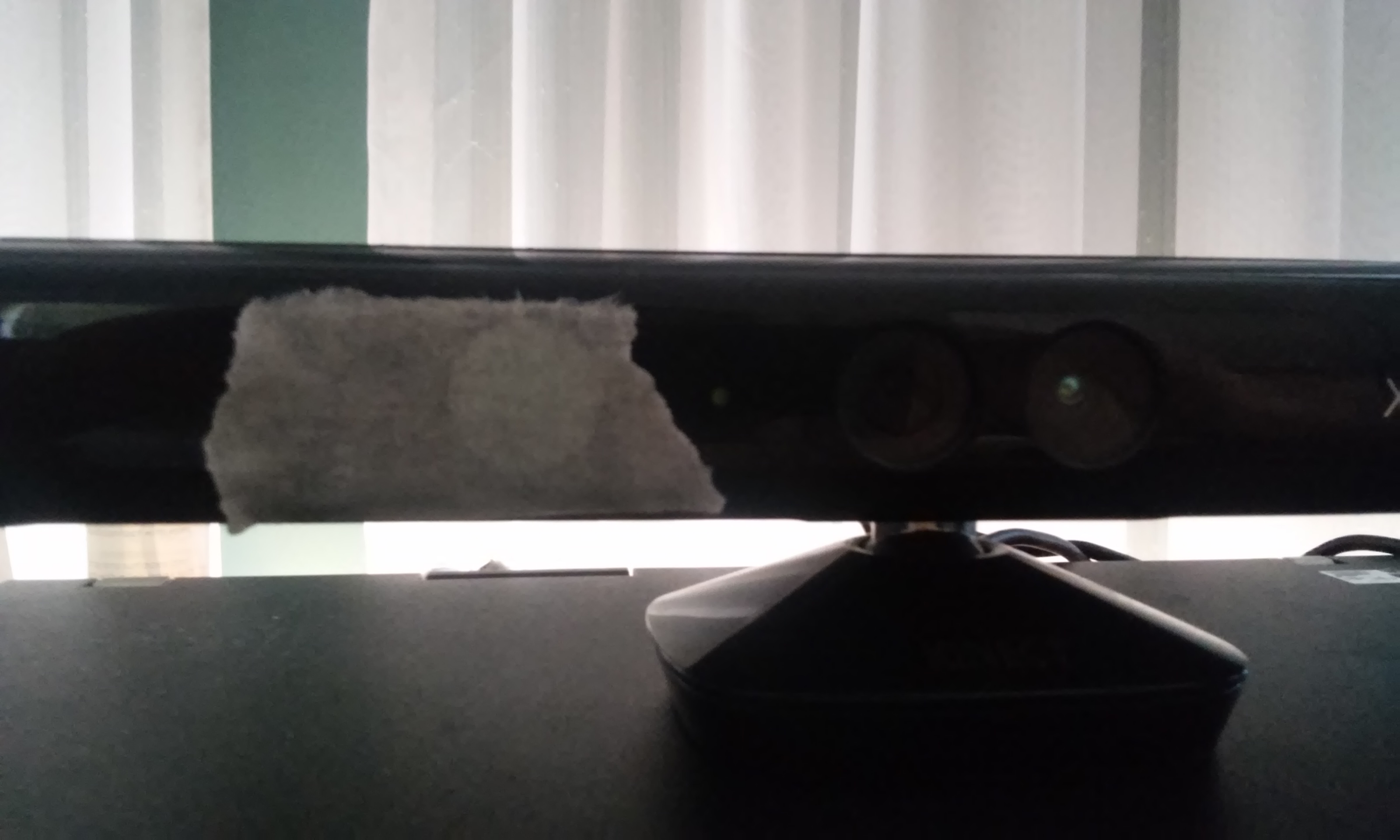
When you capture an IR video stream at the maximum resolution, as far as I know, the firmware does not allow you to adjust the gain or exposure settings. The IR laser turns out to be too bright for near-field work. So it’s best to use a static diffuser with an integrated absorber to reduce the brightness. Specifically, masking tape.

20160926_115622

The optical rig used to capture the IR video at the top of this post.

Mathematics

My implementation of the mathematics mostly follows a paper by W. James Tom, from the same University of Texas research group 4. This paper is behind a paywall, but I can summarize it here. Speckle contrast can either be done spatially (spatial variance of a single image) or temporally (variance of a location in the video stream through time) or a combination of these. I started with spatial variance.

You calculate the mean and variance of a rolling window, say 7×7 pixels. This can be done with the usual estimator for sample variance of small samples, with Bessel’s correction:

\(s^2_I = \frac{N \sum\limits_{i=1}^N I_i^2 – \left( \sum\limits_{i=1}^N I_i \right) ^2}{N \left( N – 1 \right)}\)

where \(I_i\) is the image intensity.

To find the sum and sum of squares in a given window, you iterate through all pixels in the image once, adding pixels to a stored block sum as they move into the window, and subtracting pixels as they fall out of the window. This is efficient if you store “vertical” sums of each column within the block. I think it says something about the state of scientific computing that to implement this simple moving average filter, convolution by FFT multiplication was tried first, and found to be inefficient, before integer addition and subtraction was attempted.

The variance is normalized, to produce speckle contrast \(k\):

\(k = \frac{\sqrt{s^2_I}}{\left\langle I \right\rangle}\)

where \(\left\langle I \right\rangle\) is the sample mean. From this, the correlation time as a proportion of the camera exposure time \(x\) can be found by numerically solving:

\(k^2 = \beta \frac{e^{-2x} – 1 + 2x}{2x^2}\)

For small k, use

\(x \sim \frac{1}{k^2}\)

For large k, precompute a table of solutions and then apply a single iteration of the Newton-Raphson method for each new value of k.

Finally, plot 1/x.

Results

hand-30f-ir8-vis

It’s early days. We get a big signal from static surfaces which scatter the light heavily. Ideally we would filter that out and provide an image proportional to dynamic scattering. There is a model for this in Parthasarathy et al 5. Alternatively we can do temporal variance, sometimes called TLSCI, since this should be insensitive to static scattering. After all, you can see the blood flow effect with unaided eyes in the video. The disadvantage is that it will require at least 1-2 seconds to form an image.

One of the first things I did after I connected my Kinect to my computer was wrap a rubber band around one finger and had a look at the video. The reduction in temporal variance due to the reduced blood flow was very obvious. So I’m pretty sure I’m on the right track.

Future work

So far, I have written a tool which captures frames from the Kinect and writes them to a TIFF file, and a tool which processes the TIFF files and produces visualisations like the one above. This is a nice workflow for testing and debugging. But to make a great demo (definitely a high-priority goal), I need a GUI which will show live visualized LSCI video. I’m considering writing one in Qt. Everything is in C++ already, so Qt seems like a nice fit.

The eBay seller sent me the wrong red laser, and I still haven’t received a replacement after 20 days. But eventually, when I get my hands on a suitable red laser, I plan on gathering visible light speckle images using raw Bayer data from the Kinect’s RGB camera.

References

  1. Richards, L. M., Kazmi, S. M. S., Davis, J. L., Olin, K. E., & Dunn, A. K. (2013). Low-cost laser speckle contrast imaging of blood flow using a webcam. Biomedical Optics Express, 4(10), 2269–2283. http://doi.org/10.1364/BOE.4.002269
  2. Starling MJ, Branson N, Cody D, Starling TR, McGreevy PD (2014) Canine Sense and Sensibility: Tipping Points and Response Latency Variability as an Optimism Index in a Canine Judgement Bias Assessment. PLoS ONE 9(9): e107794. http://doi.org/10.1371/journal.pone.0107794
  3. Garry A. Tew, Markos Klonizakis, Helen Crank, J. David Briers, Gary J. Hodges, Comparison of laser speckle contrast imaging with laser Doppler for assessing microvascular function, Microvascular Research, Volume 82, Issue 3, November 2011, Pages 326-332, ISSN 0026-2862, http://dx.doi.org/10.1016/j.mvr.2011.07.007.
  4. Tom, W. J., Ponticorvo A., Dunn, A. K. (2008). Efficient Processing of Laser Speckle Contrast Images. IEEE Transactions on Medical Imaging, volume 27, issue 12. http://dx.doi.org/10.1109/TMI.2008.925081
  5. Ashwin B. Parthasarathy, W. James Tom, Ashwini Gopal, Xiaojing Zhang, and Andrew K. Dunn, “Robust flow measurement with multi-exposure speckle imaging,” Opt. Express 16, 1975-1989 (2008) http://dx.doi.org/10.1364/OE.16.001975